CENTRAL AND EASTERN EUROPE 2000-2040
This forecast was prepared under the SCENES program financed by the EU.
For further data please contact NOBE.
The horizon and contents of the forecast
The forecast of the economic development of the Central and Eastern European accession countries, and selected non-accession countries covers the following 19 countries:
Poland, Hungary. Czech Republic, Slovakia, Slovenia, Croatia, Yugoslavia (Serbia and Montenegro), Romania, Bulgaria, FYR Macedonia, Lithuania, Latvia, Estonia, Russian Federation, Ukraine, Belarus, Albania, Bosnia-Hercegovina, and Turkey
For the presentation needs, the countries are divided into 6 sub-regions. The sub-regions comprise countries that share similar development patterns and development problems. Sometimes, however, the inclusion of a country into a given sub-region may be subject to controversy (e.g. Croatia shares some characteristics with the Central European countries, some with the Balkan countries; Yugoslavia can be included either into the group of Balkan countries, or countries damaged by conflicts). The sub-regions are:
Central Europe: Poland, Hungary. Czech Republic, Slovakia, Slovenia
Balkan countries: Croatia, Yugoslavia, Romania, Bulgaria, FYR Macedonia
Baltic countries: Lithuania, Latvia, Estonia
CIS: Russian Federation, Ukraine, Belarus
Countries damaged by wars/conflicts: Albania, Bosnia-Hercegovina
Turkey: Turkey
The regional forecasts (GDP per capita growth) are made only for the big and medium-sized accession
countries and Russia. Therefore, the regional forecasts are made for:Poland, Hungary. Czech Republic, Romania, Bulgaria, Russian Federation.
The classification of regions is coherent with the SCENES database and divides the accession countries into
the most likely NUTS2 units, and Russia into 12 regions reported by the national statistics.The forecast starts with the 1996 data, and estimates for the year 2000 (based on the SCENES database
and updated by the up-to-date information from the domestic sources and the EBRD projections).The forecast is made for the period 2000-2040 and presented in 10-year intervals (2000, 2010, 2020, 2030, 2040). The constant 1997 prices are used for the calculation of the GDP value according to the Purchasing Power Parity.
Level of detail of the forecast
All the forecasts are made in constant prices.
Forecasts on the national level include:
National accounts: GDP, private consumption, government consumption, gross fixed capital formation, net exports
Structure of value added and real growth rates: agriculture, industry, services
Population and employment: population, labour participation rates, unemployment rates, employment
Motorization: personal cars per 1000 inhabitants.
The regional forecasts include GDP, employment, and population.
The forecasted key variables (GDP per capita at the Purchasing Power Parity) are presented both in the US dollar values (as done by the EBRD and the World Bank) and as a percentage of the EU-15 average. For the EU a stable 2.5% yearly growth rate was assumed for the whole period 2000-2040.
The forecast is made in 3 scenarios:
Base scenario, Low scenario, High scenario
The Base scenario can be seen as generally optimistic, but realistic. The scenario assumes a relatively smooth process of the Eastern enlargement of the EU, and a successful process of the real convergence. The assumptions of the Low scenario are more pessimistic, and those of the High scenario more optimistic than those of the Base scenario.
The forecast of the economic development of the Central and Eastern European accession countries, and selected non-accession countries is based on the endogenous growth theory. The endogenous growth theory is a leading school of the economic growth theory of the 1990s (the overview of the theory can be found in: Barro R.J., Sala-i-Martin X., Economic Growth, McGraw-Hill, 1995). This theory links the long-term economic growth mainly with such factors as the human capital development, economic and political stability, economic freedom and the good legal framework for the economic activity, the private entrepreneurship and the growth-supporting policies of the State. The theory predicts the process of the conditional real convergence.
Real convergence, means an ability of a less developed economy to develop faster so that, over time, the initial gap in GDP between the less developed country and the richer countries diminishes. This principle has been observed and then empirically proven many times in history, i.e. 50 states of the United States, Japanese prefectures, and regions within the EU. In all these cases the index of convergence was at about 2% level. This means that over a longer period of time, the growth rate in poor regions is higher than the growth rate in rich regions, and the gap in economic development decreases by an average of 2% annually. From the point of view of the neoclassical economy, this can be easily explained by the following mechanism: in poor regions labour is cheap and capital relatively expensive because it is scarce (poor regions have low income, and therefore, small savings). If the capital is expensive, the marginal return resulting from its use - equal to its price - is high. That means that capital investments in a poor region bring higher returns, than in a rich region, where the capital is relatively cheap and abundant. This constitutes an incentive to move the capital from rich regions to poor regions, which in turn, leads to higher growth rates in poor regions.
In fact, high growth rates in poor regions do not require imports of capital. In the traditional models of economic growth, the neoclassical production function representing the process of transforming production factors (labour and capital) into goods and services exhibits the property of diminishing marginal productivity of production factors as their amount increases. This means that in the economy that does not have much capital, each saved and invested unit of capital gives higher production growth than in a developed economy. Therefore, there is no need to borrow capital from abroad; given the same savings rate, a less developed economy will be growing faster than a well developed economy.
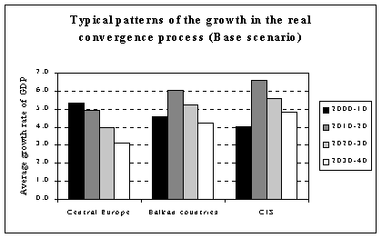
A characteristic feature of the real convergence process is that the growth of a country is the faster, the lower is the development level (obviously, if the right policies are applied). That leads to a slowdown – over time – of the growth rates when the countries approach the level of the developed countries.
Forecasting model: the growth rate
The core of the forecasts – GDP per capita growth rates - are based on the endogenous growth model of Barro, adjusted for the specifics of the transition economies.
The model is described fully in: Barro R.J., Sala-i-Martin X., Economic Growth, McGraw-Hill, 1995. The estimations were based on the cross-country sample of 97 countries, for a 10-years period.
The following formula was used for calculating the average yearly growth rates of the per capita GDP in the years 2010, 2020, 2030 and 2040:
GDP growth = -0.025 ln GDP-1 +0.0138 ENRsec +0.055 ENRtert +0.058 ln LEXP –0.315ln (GDP/HC)
+0.06 GEdu/GDP +0.07 Inv/GDP –0.06 G/GDP –0.03 INSTALecon –0.03 INSTABpol
where:
GDP-1 – GDP per capita level at the beginning of the period (log),
ENRsec – net enrollment rate, secondary education,
ENRtert – net enrollment rate, tertiary education,
LEXP – life expectancy at birth (log),
GDP/HC – GDP to the human capital ratio (log, human capital measured according to the UNIDO Human development Index, excluding the GDP per capita level),
GEdu/GDP – Government spending on education as % of GDP,
Inv/GDP – investment as % of GDP,
G/GDP – governmental consumption as % of GDP,
INSTALecon– economic instability indicator (measured by the Economic Freedom Index of the Heritage Foundation)
INSTABpol – political instability indicator (constructed by NOBE).The formula leads to the slowdown, over time, of the growth rates, as the GDP at the beginning of the period reaches the high levels in the period 2030-2040 (in the case of the most advanced countries comparable with the EU-15 GDP). For example, in the Base scenario the projected GDP growth rates of Central Europe fall from over 5% in 2000-10 (the initial p.c. GDP at 46% of the EU-15) to 3% in 2030-40 (the initial p.c. GDP at 89% of the EU-15).
As the transition is not over yet, the forecast for the years 2000-10 is a weighted average of the growth rate forecasted with the model (75%) and of the actual rate recorded in 1996-2000 (25%). In the other words, that means that the transition will still matter over the next 10 years: the economic performance of the countries that were unable to achieve a successful transformation will be still biased. One may note, that for the Central European countries the difference between the forecasted and actual rates is negligible, while for the other countries quite substantial. Therefore, the growth pattern of the less advanced reformers is different: acceleration of growth until 2020, and the lower growth only after. As the other countries are generally less developed that the Central European countries, higher growth rates may be expected after the transition is concluded (see the graph).
The most important changes in the GDP structure, measured in current prices, are included in the model assumptions. In particular, the share of fixed investment in GDP is set according to the assumed development pattern. Generally speaking, it is assumed that the optimistic development scenario requires investment to GDP ratios of 30% or more at the take-off for the fast growth. When a country reaches the development level comparable with the EU-15 the share falls to ca.20% (as in the EU). The shares of the net exports are based on the assumed current account developments. The consumption expenditures are calculated as a residual.
As far as the structure of value added (in current prices) is concerned, we assumed that the countries will follow the general direction of changes observed in the OECD countries over the period 1960-95. Under the optimistic development scenario the share of agriculture in GDP should fall from todays level of 4-6% in Central Europe and 50-60% in the countries damaged by conflicts to, respectively, 2% and 20%.
The share of the industry in GDP, quite high by the OECD standards in the majority of the countries for which the forecasts have been made, was assumed to fall to the level of between 25 and 30%. The share of services was calculated as a residual.
The real growth rates of the national accounts categories and the value added components can be calculated only if the changes in relative prices over the period of 40 years are taken into account. For example, it is a normal phenomenon that the real growth rates of the service sector are below those of the GDP. Therefore, the share of services in value added measured in constant prices should be falling. However, as the relative prices of services have been growing in all the OECD countries, despite slower growth rates the share of services in current prices was actually growing. A differnet picture can be seen in the case of industry (growth rates above those of GDP, falling relative prices, therefore falling share in value added in current prices).
In the forecast we assumed that the changes of the relative prices of various sectors of the economy and national accounts aggregates will follow the general direction of changes observed in the OECD countries over the period 1960-95 (ISB, International Sectoral Database of the OECD was used as a source of data). As in the OECD countries, the relative prices of the agriculture were assumed to fall from 1 in 2000 to 0.70 in 2040, the relative prices of industry from 1 to 0.66, and the relative prices of services to raise from 1 to 1.25. Coherent assumptions, based on the average shares of the branches of the economy in satisfying the final demand, were made about the relative prices of the national accounts aggregates.
Therefore, the share of the industry (demand component) i in GDP in constant prices was calculated from the formula:
shareiconst.prices = shareicurrent.prices/ (Pi/PGDP)
where:
shareiconst.prices – share in constant prices, shareicurrent.prices – share in current prices,
Pi/PGDP – realtive prices measured against the GDP deflator.If the industry (demand component) had falling relative prices (Pi/PGDP <1), the share in constant prices is higher than the share in current prices, that implies higher real growth rates.
With the calculated shares in constant prices, and the real GDP levels, it was possible to calculate the real levels of the value added by sectors and the final demand components in the years of the forecast and the growth rates.
The forecast of the population trends in the Central and Eastern European accession countries, and selected non-accession countries covers the following 19 countries:
Poland, Hungary. Czech Republic, Slovakia, Slovenia, Croatia, Yugoslavia (Serbia and Montenegro), Romania, Bulgaria, FYR Macedonia, Lithuania, Latvia, Estonia, Russian Federation, Ukraine, Belarus, Albania, Bosnia-Hercegovina, and Turkey
Instead of constructing simple demographic models for those countries, which would have to be based on the rather scarce data on population cohorts and a set of uniform assumptions about demographic coefficients, it has been decided to use the most recent forecast of population of the United Nations (World Population Prospects, The 1998 Revision, Volume II: Sex and Age, United Nations, New York 1999). The UN population forecast covers three variants distinguished by different assumptions on fertility rates. For the SCENES project the medium variant was selected.
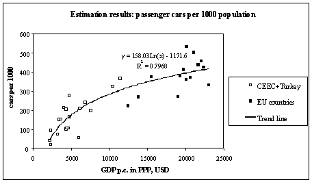
The level of motorization (passenger cars per 1000 inhabitants) was forecasted with the use of the regression linking this parameter with the GDP per capita levels (measured at PPP). The regression was based on the sample of countries including the EU-15 member states (without Luxembourg) and the 19 countries for which the forecasts were made.
The graph presents a logarithmic trend line we decided to use:
The logarithmic trend line reflects the fact of the existence of a possible saturation level at 400-500 cars per 1000 inhabitants achieved by the countries with the GDP p.c. levels of above 20 000 –25 000 USD.

The following assumptions were made in the three scenarios of the economic development of the Central and Eastern European accession countries, and selected non-accession countries.
Education (secondary and tertiary enrolment ratios):
Base scenario: Central Europe, Baltic and CIS countries reach the levels of the EU-15 by the year 2040, Balkan countries 20% below, damaged countries 30% below, Turkey 20% below.
High scenario: Central Europe, Baltic and CIS countries as in the base scenario, Balkan countries 10% below, damaged countries 20% below, Turkey 10% below.
Low scenario: all the countries 10% below the Base scenario.Life expectancy at birth:
Base scenario: Central Europe, Baltic and CIS countries reach 73-74 years by the year 2040, Balkan countries 72, damaged countries 72, Turkey 70.
High scenario: all the countries 5% above the Base scenario.
Low scenario: all the countries 5% below the Base scenario.Government spending on education as % of GDP – no change, only in Turkey increase from 2% to 4% in the Base and High scenario, in damaged countries from 4% to 5%.
Investment share in GDP:
Base scenario: Central Europe: peak - 30% - in 2010, fall to 20% in 2040, Baltic countries: 30% in 2010, fall to 25% in 2040, CIS countries: 30% in 2020, fall to 25% in 2040, Balkan countries 30% in 2020, fall to 27% in 2040,, damaged countries 30% in 2030, fall to 27% in 2040, Turkey 30% in 2010, fall to 20% in 2040.
High scenario: 2 percentage points above the base case.
Low scenario: reaching the peak delayed by 10 years.Governmental consumption share in GDP: calculated under the assumption of the governmental consumption growth rate of 80% of the GDP growth.
Economic instability (Economic Freedom index):
Base scenario: the index falls by 2040 to 2 (the average current EU-15 level) in Central Europe, Baltic, Balkan countries and Turkey, to 2.5 (current Central European level) in CIS and damaged countries.
High scenario: the index falls by 2040 to 1.8 (the current Irish level) in Central Europe, Baltic, Balkan countries and Turkey, to 2.2-2.3 (current EU-15 level) in CIS and damaged countries.
Low scenario: the index falls by 2040 to 2.2 (the current level in the least liberal EU countries) in Central Europe, Baltic, Balkan countries and Turkey, to 2.7-2.8 (current Turkish level) in CIS and damaged countries.Political instability:
Base scenario: Central Europe and Baltic countries join the EU around 2005 and EMU by 2010, Balkan countries and Turkey 10 years later, damaged and CIS countries achieve the high level of the political stability by 2020-2030.
High scenario: similar in Central Europe, Baltic countries, and Turkey, 5 years delay in the accession of the Balkan countries, 10 years faster political stabilization in damaged and CIS countries.
Low scenario: accession of Central Europe and Baltic countries delayed by 5 years compared to the Base scenario, accession of Turkey and Balkan countries by 10 years; damaged and CIS countries still politically unstable by the year 2030, and only partly stabilized by 2040.

Economic development of a country is characterized by unequal regional development: some regions develop at a higher pace than others. Theory of modern economic growth explains differences in the speed of regional development in terms of the real convergence. Regions with higher GDP per capita tend to grow slower than regions with lower GDP per capita. A particular difficulty with the application of the pure convergence concept to explain regional differences in economic development of transition economies is that the differences tend to intensify during periods of accelerated structural changes occurring in the period of transition. On the other hand the prosperity of regions depends on the ability of regions to adopt to the conditions of the market economy, which is an endogenous factor for the region. Closer look at these phenomena has a very practical meaning, since understanding of them may help to stimulate future development of regions.
Regional forecasts prepared for the project were therefore based on the formal model, which directly explained deviations of regional GDP per capita from the country average level. The model was originally developed in order to study differences in regional development of Poland in the transition period and factors which influence them. In a sense the model is consistent with the endogenous growth models, used to forecast economic growth at a country level.
In general, among factors stimulating regional development in the model economic factors, often called hard factors (natural resources, labour and capital resources, traditional infrastructure as well as capital outlays related to these resources -increasing endowment and efficiency of use) and non-economic factors – called also soft factors are distinguished. The latter category comprises factors which first of all spur localization decisions. To this category of factors belongs a cultural and historical heritage (which increases attractiveness of a region and is the basis of the work ethos) and investments rising up the living conditions in the region (ecological environment, leisure time facilities etc.). Soft factors decide, that among regions of comparable economic factors endowment some are developing faster then others.
Combination of all those factors appears in the formal model, which instead of explaining directly economic growth of regions by the initial GDP per capita, rather links regional disparities (relations of regional GDP per capita to the country average) and selected hard and soft factors. The model has following advantages:
it explains directly regional disparities (GDP per capita at the level of a country = 100), hence
it has a built-in constancy of regional and national GDP forecasts;the set of explanatory variables contains variables, which allow for making a distinct scenario
assumptions about the factors, which are likely drive regional disparities.the presence of the initial regional disparities in the set of explanatory variables makes the model
a dynamic one.The basic disadvantage of the model is that it is rather data demanding. To overcome the difficulty we assumed parameters of the model at the “Polish” level. In order to simplify regional scenarios, assumptions have been restricted to the following:
only drivers of regional disparities are education and infrastructure; other variables were assumed
to be equally distributed amongst regions.education disparities were usually explained by the share of population with secondary and tertiary
(sometimes the tertiary only) in region relative to the share calculated at the country level;infrastructure density indicator described the road and/or rail network density in region relative to
the country level;base scenario assumes that regional disparities in education and infrastructure saturation would
remain stable or would slowly increase;in low scenario regions which are better off would attract more infrastructure and would faster
increase the quality of human capital (education), thus leading to the increase in regional disparities;high scenario assumes the opposite: active regional policy at country and regional level would help
to allocate more infrastructure investment to poorer regions and upgrade the quality of human capital
in those regions, thus reducing regional disparities.The specification of the model and values of estimated parameters are presented in the table. All variables are expressed in relation to the appropriate country average levels.
Factors
Estimated impact
Human capital
Level of education
29.3%
Demogr. character istics
0.0%
Population mobility
24.3%
Work ethos
0.0%
Cultural background
0.7%
Urbanization
0.4%
Initial development
Initial GDP
14.6%
Initial infrastructure
0.0%
Economic structure
Role of agriculture
0.0%
Role of industry
3.5%
Role of services
2.8%
Infrastructure development
5.2%
Capital city
2.9%
Regional centers
0.1%
Resilience of local government.
16.2%
Environmentally unfriendly economic structures
0.0%
100.0%
Source: Czyżewski, Orłowski, Zienkowski "Factors Stimulating and Disadvantaging Economic Development of Regions", Research Bulletin RECESS, 3/1995